Unlearn Machine Learning - Building SGD from scratch

Shishya: Good morning, Professor. I have finished Andrew NG's machine learning 
course on Coursera. And now that I have a grip over a few algorithms, I'm ready to 
build a ML model. 
 

Guru: Well, well. That's not what I'm here for. You have kaggle.com and various other 
sites for that. I'm here to teach you something different. You just said you learnt about 
a few ML algorithms. Can you name any?

Shishya: Oh yes. I learnt about linear regression, support vector machines, stochastic 
gradient descent, clustering algorithm, random forests, etc.

Guru: Hold on. You just said you learnt these algorithms. But let me take some of your time, 
and help you build whatever descent algorithm it is, all by yourself. Let us unlearn those 
algorithms for a while, and build it from scratch.

Shishya: Wow. Really? Interesting........ But, no. I don't like math, especially calculus and stuff.

Guru: Haha... don't worry, my boy. You are just in the right place, and get ready for a 
adventurous ride.

Shishya: Okay. I just hope, this isn't another math tutorial class.

Guru: Let us look at an age old example of predicting the price of a new price from housing data:

Now, given historical housing data the task is to create a model that predicts the price of a new house 
given the house size.

Lets plot the above data

Shishya: Alright. I know what we should do next. We have to come up with a

simple linear model, where we fit a line on the historical data, to predict the price of a new house 
(Ypred) given its size (X). So, we need to find a line with optimal values of a,b (called weights) that 
best fits the historical data by reducing the prediction error and improving prediction accuracy.

So, our objective is to find optimal a, b that minimizes the error between actual and predicted values 
of house price

Guru: Yes. you are right there. But where do we start from. Any guesses?

Shishya: Of the many problems I have solved, I have seen almost all of the problems start with 
assuming random values for input parameters, i.e., in our case it is 'a' and 'b'.

Guru: Correct. Looks like we are on the same page. Now, before I start off any further, I would like you 
to keep the below points in mind.

1. We will be scaling our data to a smaller range, without disturbing its variation and distribution.

2. We might have to go back and tweak our equations

3. We will be progressing towards our model in smaller, repetitive but correct steps.

We are pretty sure our random values of a and b, will give us wrong output. How do we mend the 
values of a and b, so that we get an appropriate output. What should be the basis for correcting 
the values of a and b. William Schwenck Gilbert, a legendary dramatist of 1850s said 
"Let the punishment fit the crime". So what crime did the random values of a and b commit. 
How do we measure that crime, to determine the punishment? Let's rewrite our new values 
of a and b as

na = a - pa 

where na = new value of a

pa = some punishment for a

Similarly,

nb = b - pb

Shishya: Haha, its a no-brainer. Lets calculate the inaccuracy of our best fit line. This can be done by 
computing the sum of all the differences between the actual house price and the predicted house 
price (best fit line)

Guru: Okay, hang in there. Before you proceed, I wanted to remind you of one of the points about 
scaling our data. We have to standardize the data as it makes the optimization process faster. 
The reason should not be hard to figure out. Imagine your computer crunching numbers in the 
range of 1-10,000 vs numbers in the range of 0-1. When you can get to reduce the range of your 
data-set without affecting the modeling, its always better, as the CPU/GPU is comfortable dealing with 
lesser range.

Shishya: Yes, I got it. We need to scale down our data set to the range of 0-1 for both house prices
 and house sizes. That's easy. Divide each value in house size by the maximum value of house size 
(in our case, it is 2450), and similarly for house price.

Guru: Really, will that suffice? Here, have a look at this table below.

Shishya: Hmm. Got it. The immediate thought that occurred to me is to divide each of house size 
values by its maximum value i.e., 2450 in our case. But, when we look at the lowest point in the scaled 
house size, it is 0.44 (1100/2450). However, we would like to stretch the lowest point to 0 and highest point to 1.

And I see that the next column with "min max scaling", the values are stretched out to as low as 0 and 
as high as 1, which is what we required. Professor, could you please help me in figuring out how you 
came up with min max scaling.

Guru: Haha, there you go. You are on the right track, my boy. Just an heads up, in machine learning, 
there are two standardization techniques  - z score standardization and min-max scaling. 
In this example we have used min-max scaling. Anyways lets look at the formula for min max scaling. 

Looking at the formula, we have a common denominator, the farthest value from Xmin, and the 
numerator denotes how far each of the values of X are from the Xmin, which naturally gives an 
output range of [0,1]. Just try plugging in the lowest value X=1100 and highest value X=2450 in the 
equation and check for yourself.

Shishya: Yep, got it. Okay, now that I have understood why and how normalization works, lets get 
back to our main problem. 

Guru: Good. From here on, lets get a bit technical. Let's us try to define the crime in terms of 
mathematical equation. Use the below graph to define that equation.

 

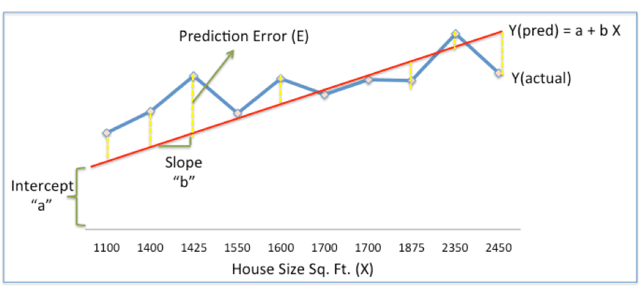
Shishya: The first thought we get on looking at the above graph, is to add up the differences 
(between Y-actual and Y predicted) at the various size points (X-coordinate). But, we face 
the issue of negative errors. No problem with that, lets take the absolute value and add it up. 

So, Error = | (Y - Yp) | 

[Shishya hands over this table to professor]

Guru: Hmm, not bad. But, not the correct step either. Anyways, not a problem. Lets move ahead. 

Well, now that we have a measure of how much error is produced due to random nature of a and b, 
 pa (some punishment for a) should be calculated on the basis of this error. Now one thing we are 
sure of is, pa = function(error). What is that magic function. What should this function do?

Shishya:

1. It has to measure the total error produced by each unit of 'a' ('a' is a finite value on Y axis of the graph)

2. It has to measure the individual contribution of 'a' and 'b' towards the error

Guru:

Can we rewrite the first point as "it has to measure the rate of change of total error with respect a".

[Professor gives a short pause]

Doesn't it sound like the definition of a derivative - "The derivative is the instantaneous rate of change 
of a function with respect to one of its variables."

Shishya: Yes, correct. 
 

Guru: Lets Welcome your beloved high school friend, Mr. Calculus. 

If we differentiate total error with respect to a and b, we get to see how much each unit of 'a' and 'b' 
had contributed to the total error. But doesn't something smell fishy? How do we differentiate with 
respect to both a and b? We know that our total error is function of both a and b. But we need to 
get two values pa and pb. And this is why partial differentiation comes into the picture.

Shishya: Wavvv. Calculus is truly my dear friend. Cool, now that we know that function is nothing 
but a partial derivative of our total error with respect to a and b. Lets me try out that. 

[Shishya hands over the below sheet of paper]

Guru: Impressive. I'm sure you would have got an S grade in Engineering mathematics. But look at the
derivatives. Do they look like something useful? How do you plan to use these derivatives to calculate
the correction value? Can we redefine our error function in such a way that derivative is meaningful? 
The main culprit I see is the modulo function ? Can you come up with something so that we can get 
away with the modulo function?

Shishya: We can square the difference right.? We brought in the modulo because of negative difference 
values. No harm right.? We still are retaining the error measurements.

Guru: That's correct. You should also multiply the error function by 1/2. As derivative of the squared 
function will result in value that is a factor of 2. Now your error function looks something like this.

Tweaked Error Functon = ½ Sum (Actual House Price – Predicted House Price)2

=  ½ Sum(Y – Ypred)2

The above error function is nothing but, SSE (Sum of Squared Errors). Now, can you calculate the 
partial derivative of SSE with respect to a and b.?

[Shishya hands over another sheet of paper]

Now that we have some equations, lets use them in our housing data table.

Guru: Now, remind yourself of my third point, that I had told you at the beginning. We need to move in 
small steps. We are not going to reach to the correct value in one go. We will iterate in small steps 
towards the most appropriate value. Hence we multiply pa and pb by something called as learning rate (r)
, which minimizes the values of pa and pb

Lets look at the corrected value of a and b.

New a = a – r * ∂SSE/∂a  = (0.45-0.01) * 3.300 = 0.42

New b = b – r * ∂SSE/∂b = (0.75-0.01) * 1.545 = 0.73

here, r is the learning rate = 0.01

Plugging in the new values of a and b, you get

Shishya : And this is exactly what Stochastic gradient descent is all about right? Since we started 
our problem with random values, the word 'stochastic'. And, I see that we are descending interms 
of our SSE values,from 0.677 to 0.553. Hence the name. Now, let me calculate another set of a and b
 and check the SSE.

Guru: Hold on boy, you have got it. There are number of libraries like sklearn to do that for you. 
Now that you have built the SGD algorithm from scratch and understand its nitty-gritties, do share it 
with your friends :)